
Overview
This use case applies Seasonal ARIMA (SARIMA) modelling to a time series with a clear long-term trend and recurring seasonal structure. The workflow first diagnoses the observed series, then introduces differencing and seasonal terms to remove non-stationary behaviour, estimates the model, and finally validates whether the remaining residuals behave like unpredictable noise.
Although the example is illustrated with monthly airline-passenger data, the same architecture is directly applicable to electricity demand, commodity consumption, industrial production, transport activity and other economic or market series where both trend and seasonality matter. The goal is to turn repeated historical patterns into a statistically validated forecasting process that can support planning and risk decisions.
Business relevance
- Forecast seasonal demand or market activity when both trend and recurring periodic effects are present.
- Separate persistent growth from seasonality so forecasts are not driven by raw historical levels alone.
- Validate whether the fitted model has removed meaningful autocorrelation from the residuals.
- Support capacity planning, procurement, budgeting and scenario analysis with an explicit time-series model.
- Provide a repeatable forecasting framework that can be recalibrated as new observations arrive.
Solution
The solution is to use the structure visible in Figure 1 to specify a forecasting model that explicitly separates trend and seasonality. The series rises over time while repeating a very similar annual pattern, and the amplitude of the seasonal swings also grows as the level of the series increases. A simple linear forecast would miss those recurring peaks and troughs, while a non-seasonal ARIMA model would fail to capture the 12-month dependency. The SARIMA specification therefore combines ordinary differencing with seasonal differencing and seasonal moving-average terms.
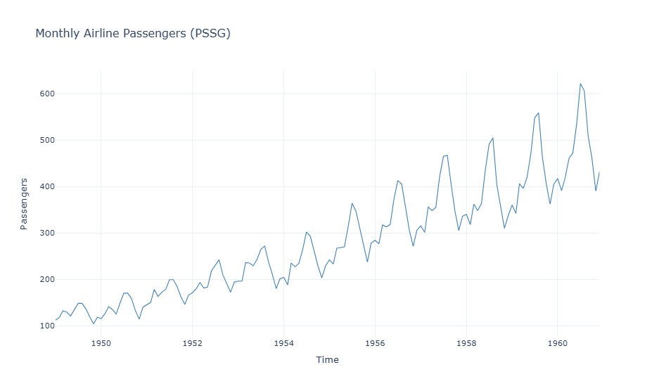
Figure 2 is the validation step. The standardised-residual panel checks whether large unexplained shocks remain; the residual ACF checks whether predictable serial correlation is still present; the histogram and QQ plot show whether the residual distribution departs materially from the assumptions used by the model. The visible seasonal ACF spike and the extreme residual observations indicate that the fitted specification is informative but not perfect, so those diagnostics should be treated as model-governance evidence rather than ignored.
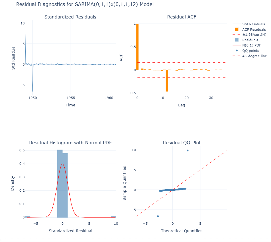
Used operationally, the framework can generate rolling forecasts for electricity demand, commodity volumes or other seasonal business series and then monitor the same residual diagnostics after every recalibration. If autocorrelation or extreme residual behaviour reappears, the model can be respecified before its forecasts are used for capacity, procurement or risk decisions. Figure 1 therefore tells us what structure must be forecast, while Figure 2 tells us whether the chosen model has captured that structure well enough to be trusted.