Kalman Filtering | Proxima Alpha

Overview

This use case applies a local-linear-trend Kalman filter to a univariate macroeconomic series treated as log(GDP). The model represents the observed series as a noisy measurement of two hidden states: a latent level and a latent slope. Maximum-likelihood estimation determines the process and observation variances, after which the Kalman filter recursively updates the state estimates as new observations arrive. A Rauch-Tung-Striebel smoother then uses the full sample to refine the latent trend and slope, and the final smoothed state is used for forecasting and Monte Carlo simulation.

The workflow is useful because many economic and market series mix persistent signal with short-run noise. Instead of applying a fixed moving average, the Kalman framework continuously decides how much weight to give to the model versus each new observation, producing an interpretable decomposition and explicit uncertainty bands.

Business relevance

Extract a smooth latent trend and growth signal from noisy macroeconomic or market data.
Update forecasts recursively as new data arrives without re-estimating the entire history from scratch.
Separate signal from measurement noise and quantify state uncertainty at each point in time.
Use filtered and smoothed states as inputs to macro monitoring, scenario design, forecasting or risk models.
Identify changes in latent slope that may indicate acceleration, slowdown or local regime shifts.

Solution

The solution is to represent log(GDP) with a local linear trend state-space model in which the hidden state contains level and slope. The estimated observation and slope-noise variances are extremely small, while level noise is also low, so the filter interprets the series as highly persistent and close to deterministic. That explains why the filtered and smoothed trend closely track the observed data and why forecast intervals remain relatively tight.

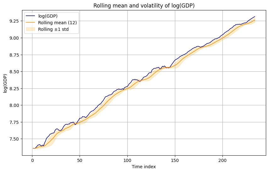
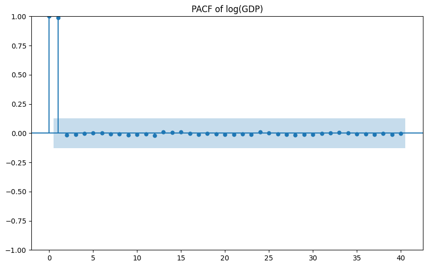
Figure 1. Rolling mean and volatility of log(GDP), illustrating the strong upward trend and relatively narrow local dispersion.

The visual diagnostics reinforce that interpretation. Figure 1 shows a steadily rising log(GDP) path with a rolling mean that follows the level closely; Figure 2 shows that most of the partial dependence is concentrated at the first lag. The full workflow then uses innovations, Kalman gains and residual diagnostics to test whether the signal extraction is behaving as expected. Standardised residual variance is close to one, but the very low Jarque-Bera p-value indicates non-normal residuals, so the Gaussian model is probably too confident in the tails.

Figure 2. PACF of log(GDP), showing a dominant first-lag effect and little additional partial correlation at higher lags.

Forecasting extends the final smoothed state forward for 12 periods. The first forecasts continue the positive trend with narrow intervals, and 300 Monte Carlo paths produce a similarly tight distribution. Operationally, this gives decision-makers a clean latent trend and an updateable forecast, while the source analysis correctly flags the next improvements: heavier-tailed observation errors, a less restrictive measurement-noise assumption, additional cyclical states and formal structural-break tests.