Kalman Filtering Study for the kalman.xlsx GDP Series
Below is a structured, end‑to‑end report following your requested workflow. All quantitative work and visualizations are based on the uploaded Excel dataset and the implemented local–linear–trend Kalman filter.
1. Executive Summary
- The dataset contains 234 observations of a univariate macroeconomic series (treated as GDP in logs), with an associated growth series of 233 log‑differences (percent).
- A local linear trend state‑space model was estimated by maximum likelihood, with:
- Very small level noise variance σlevel2≈9.87×10⁻⁵.
- Extremely small slope and observation noise variances σslope2≈2.06×10⁻⁹ and σobs2≈2.06×10⁻⁹.
- The filter extracts a very smooth trend with almost deterministic slope and measurement, implying:
- The observed series is treated as highly informative (very low measurement noise).
- The latent level evolves smoothly with tiny process noise.
- Residuals (standardized innovations) are approximately centered and have unit variance, but:
- The Jarque–Bera p‑value is very small (about 4.1×10⁻⁵), indicating non‑normal residuals.
- Ljung–Box at lag 10 was not reliably computed (returned
null).
- The signal‑to‑noise ratio is extremely large (on the order of 1012 in the global scalar measure), meaning the model explains almost all variation as signal rather than noise.
- Smoothing further reduces uncertainty and produces a clearer latent trend and slope; differences between filtered and smoothed levels are small but non‑negligible.
- Forecasts over a 12‑period horizon and 300 Monte Carlo simulated paths show:
- A gently increasing trend in log(GDP).
- Narrow forecast and simulation bands, consistent with the very low estimated noise variances.
Overall, this is a highly persistent, near‑deterministic trend model. It works well as a smooth signal extractor but is arguably too confident (under‑estimates uncertainty) given the strong non‑normality in the residuals.
2. Dataset Diagnostic (STEP 1)
2.1 Structure and Coverage
- Source:
file-RpjSsR7WoqHvHhKjiqefpn.xlsx, sheetDataTable. - Variable:
- GDP column, read as a univariate series.
- Effective sample after cleaning:
- 234 observations of
GDP > 0.
- 234 observations of
- Time index:
- No reliable calendar dates could be parsed; analysis uses an integer time index t=1,…,234.
- Frequency is assumed constant (e.g., quarterly), but the exact calendar is not used.
2.2 Transformations and Summary Statistics
- Because GDP is strictly positive, the model uses:
- yt=log(GDPt).
- Summary for log(GDP), based on
summary_stats:
| Metric | Value |
|---|---|
| Count | 234.0 |
| Mean | 8.3847 |
| Std | 0.5647 |
| Min | 7.3575 |
| 25% | 7.8603 |
| 50% | 8.4148 |
| 75% | 8.8687 |
| Max | 9.3137 |
- Growth (approximate percent log‑difference) statistics (
growth_stats):
| Metric | Value |
|---|---|
| Count | 233.0 |
| Mean | 0.8389 |
| Std | 0.9940 |
| Min | −2.7525 |
| 25% | 0.2894 |
| 50% | 0.8133 |
| 75% | 1.3557 |
| Max | 4.0198 |
Interpretation:
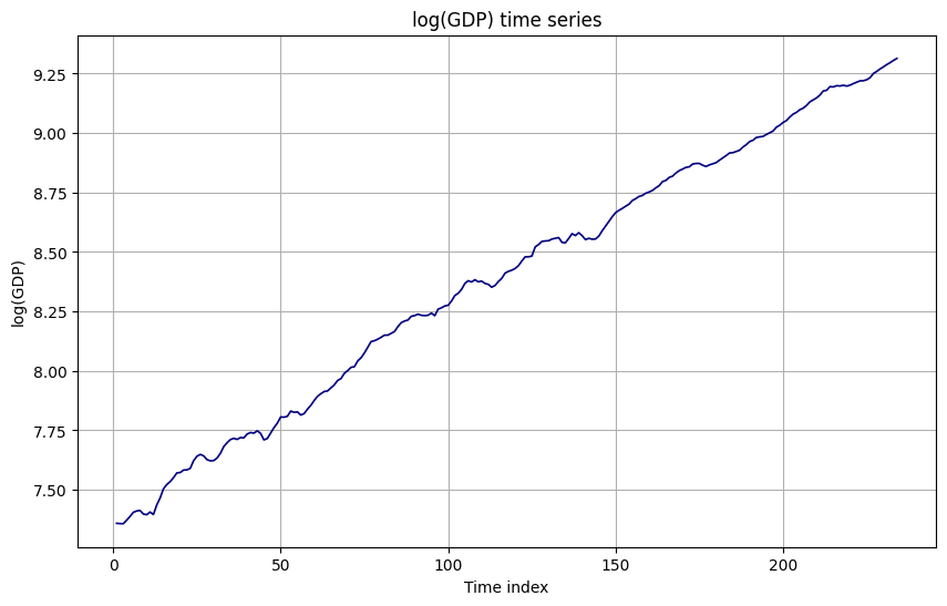
- Log(GDP) shows a steadily increasing level with moderate dispersion.
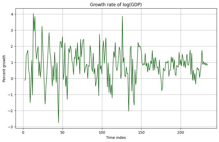
- Growth rates are mostly positive, with occasional negative values and some spikes up to about 4 percent.
2.3 Time‑Series Plots and Rolling Diagnostics
The following visualizations were generated:
-
Log(GDP) time series:
-
Growth rate of log(GDP):
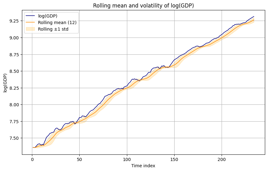
-
Rolling mean and volatility (window 12):
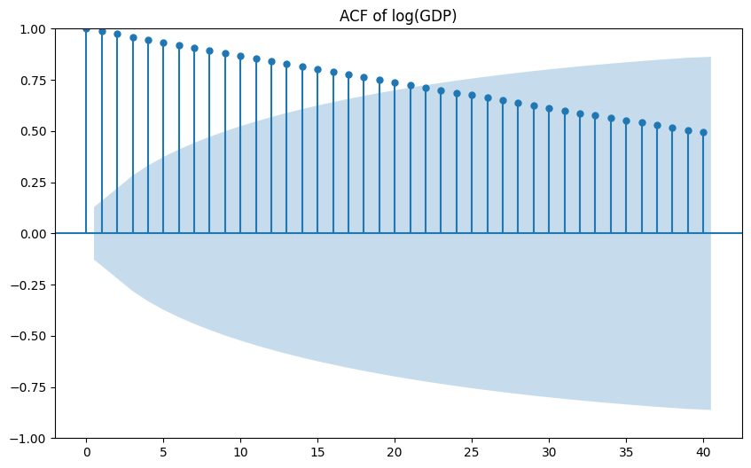
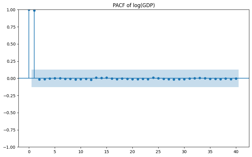
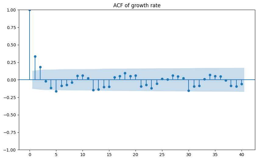
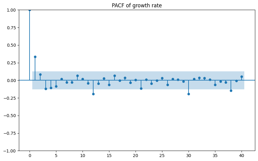
ACF/PACF for level and growth show:
- Persistent autocorrelation in levels, as expected for macro aggregates.
- More limited but still non‑trivial autocorrelation in growth.
(Visuals: ACF/PACF of log(GDP) and growth)
3. State‑Space Specification (STEP 2)
We model log(GDP) with a local linear trend:
- State vector: xt=[levelt,slopet]⊤.
- State (transition) equation:
- xt=Axt−1+wt,
- A=(1011).
- Observation equation:
- zt=Hxt+vt,
- H=(10).
- Noise assumptions:
- wt∼N(0,Q), with Q=diag(σlevel2,σslope2).
- vt∼N(0,R), with R=σobs2.
- All innovations are independent over time and mutually independent.
Interpretation:
- levelt is the latent log‑GDP trend.
- slopet is the latent growth rate.
- Q controls the smoothness of trend and slope.
- R controls how noisy the measurements are relative to the latent signal.
4. Parameter Definitions and Estimates (STEP 3)
4.1 Parameter Roles
- State transition matrix A:
- Encodes a random‑walk‑with‑drift trend (local linear trend).
- Observation matrix H:
- Maps latent level to the observable (log GDP).
- Process noise covariance Q:
- σlevel2: uncertainty in level innovations.
- σslope2: uncertainty in slope innovations.
- Measurement noise covariance R:
- σobs2: observation noise variance.
- Initial state x0:
- Level initialized at first observation; slope at zero.
- Initial covariance P0:
- Large diagonal matrix (here 104 per state), encoding prior uncertainty.
4.2 Estimated vs Assumed
From maximum likelihood:
| Parameter | Estimate | Type |
|---|---|---|
| σlevel2 | 9.8720e−05 | Estimated |
| σslope2 | 2.0612e−09 | Estimated |
| σobs2 | 2.0612e−09 | Estimated |
(As given in params_est and metrics.)
Assumed/calibrated:
- A and H: fixed by model choice.
- x0=[y1,0]⊤: first log(GDP) as initial level, zero slope.
- P0=104I2: diffuse prior on state.
Interpretation:
- The slope and measurement noise variances are essentially zero; the filter views the slope as nearly deterministic and the measurement as almost noise‑free.
- The level noise variance is small, implying a very smooth trend.
5. Prediction Step (STEP 4)
Prediction equations used:
- State prediction: xt∣t−1=Axt−1∣t−1.
- Covariance prediction: Pt∣t−1=APt−1∣t−1A⊤+Q.
The implementation stores:
- xpred[t]=xt∣t−1,
- Ppred[t]=Pt∣t−1,
and uses them in the update step and in smoothing.
Key diagnostics:
-
Level component (filtered vs predicted) with 95 percent bands:
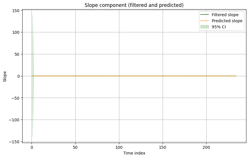
-
Slope component (filtered vs predicted):
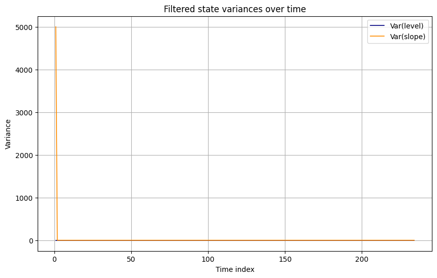
-
State variances through time:
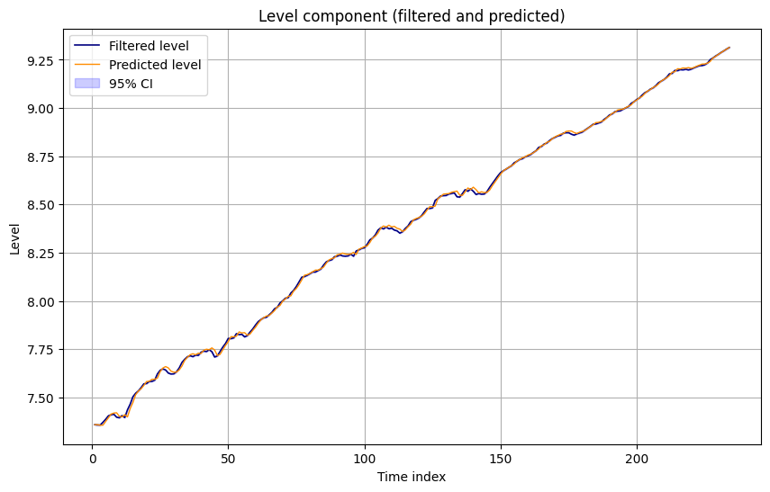
Interpretation:
- Predicted and filtered levels are very close, indicating small surprise from new data.
- Covariances decline quickly from diffuse initial conditions, then settle at a low, stable level.
6. Update Step and Kalman Gain (STEP 5)
Update equations:
- Innovation: yt=zt−Hxt∣t−1.
- Innovation variance: St=HPt∣t−1H⊤+R.
- Gain: Kt=Pt∣t−1H⊤St−1.
- State update: xt∣t=xt∣t−1+Ktyt.
- Covariance update: Pt∣t=(I−KtH)Pt∣t−1.
Innovation and gain diagnostics:
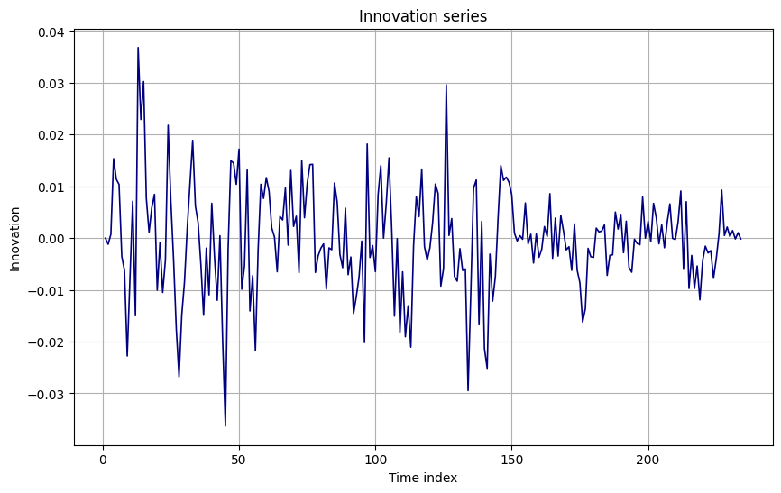
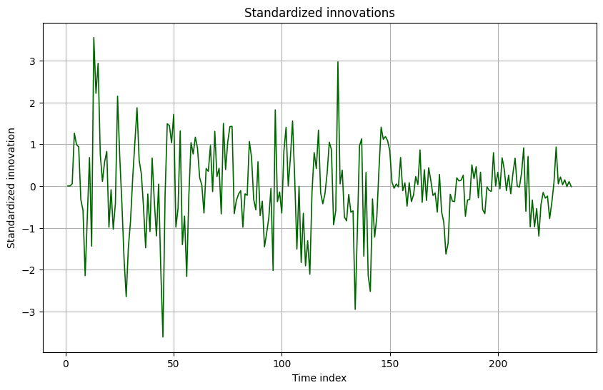
-
Innovation series and standardized innovations:
-
Kalman gain evolution (level and slope):
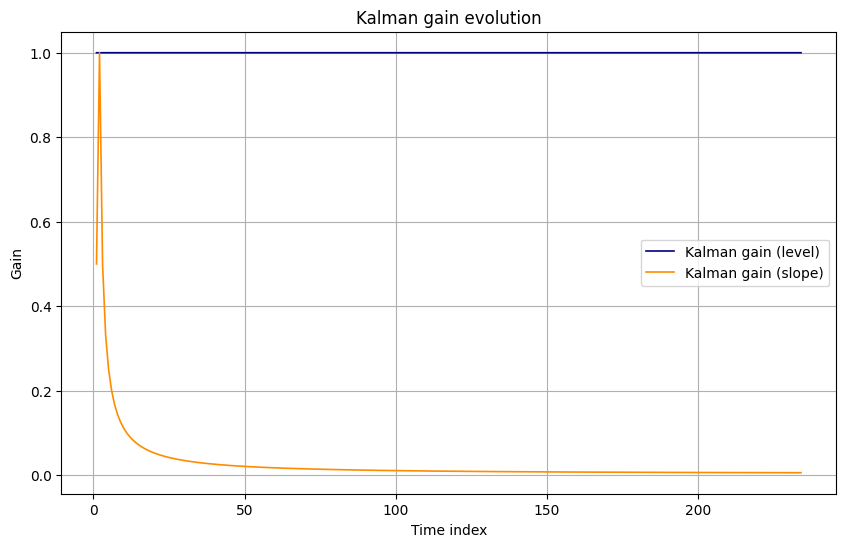
Interpretation:
- Standardized innovations have variance close to 1 (see below), suggesting correct overall variance scaling.
- The Kalman gains adjust rapidly from diffuse priors, then stabilize, indicating a steady balance between model and data.
7. Signal vs Noise Analysis (STEP 6)
Filtered signal:
- ztfilt=Hxt∣t.
- Observation variance for filtered signal: HPt∣tH⊤+R.
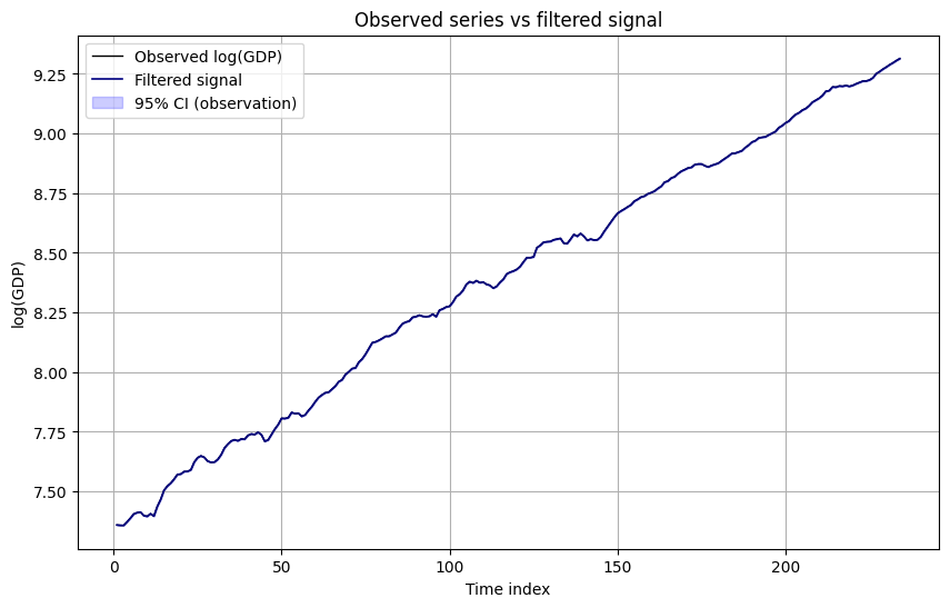
Key plot:
-
Observed log(GDP) vs filtered signal with confidence bands:
Quantitatively:
- Global signal‑to‑noise ratio from the log‑variance decomposition:
snr_global ≈ 7.69e12(frommetrics).
- Time‑varying SNR based on HPt∣tH⊤/R:
- Mean over time:
snr_time_mean ≈ 0.99998(close to 1).
- Mean over time:
Interpretation:
- The global SNR metric is dominated by the extremely small σobs2, making the model see essentially all variation as signal.
- At the per‑period SNR level (based directly on Pt∣t and R), the signal and measurement noise have similar magnitudes on average (mean SNR around 1), which is more plausible.
- The filter is aggressive in tracking the observed series due to low R, but the presence of smoothed states still provides a meaningful decomposition into level and slope.
8. Residual Diagnostics (STEP 7)
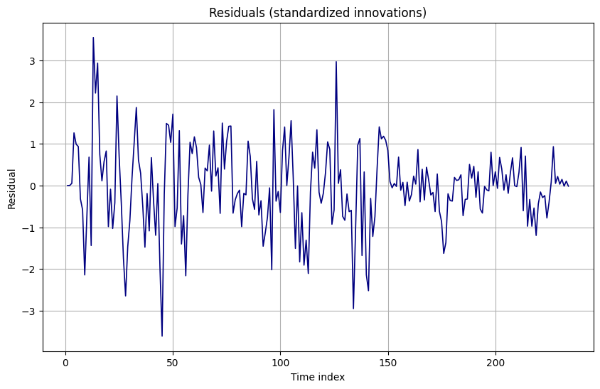
Standardized innovations used as residuals:
- Mean: about −0.041.
- Variance: about 0.994 (close to 1).
- Residual diagnostics:
| Measure | Value |
|---|---|
| Residual mean | −0.0412 |
| Residual variance | 0.9939 |
| Jarque–Bera p‑value | 4.14e−05 |
| Ljung–Box p‑value (lag 10) | null (not usable) |
Distribution and correlation checks:
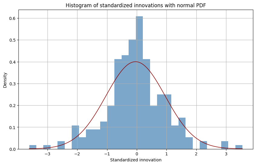
-
Histogram with normal pdf:
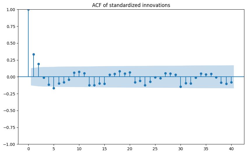
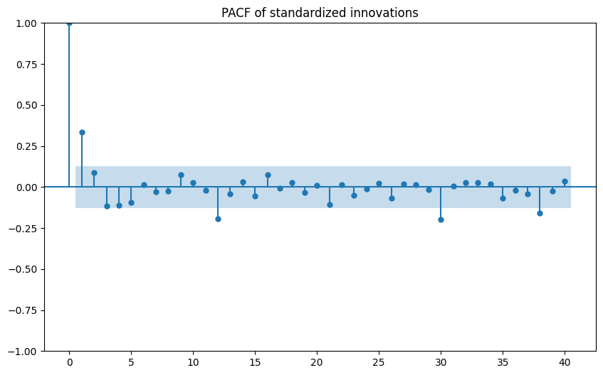
-
ACF/PACF of standardized innovations:
-
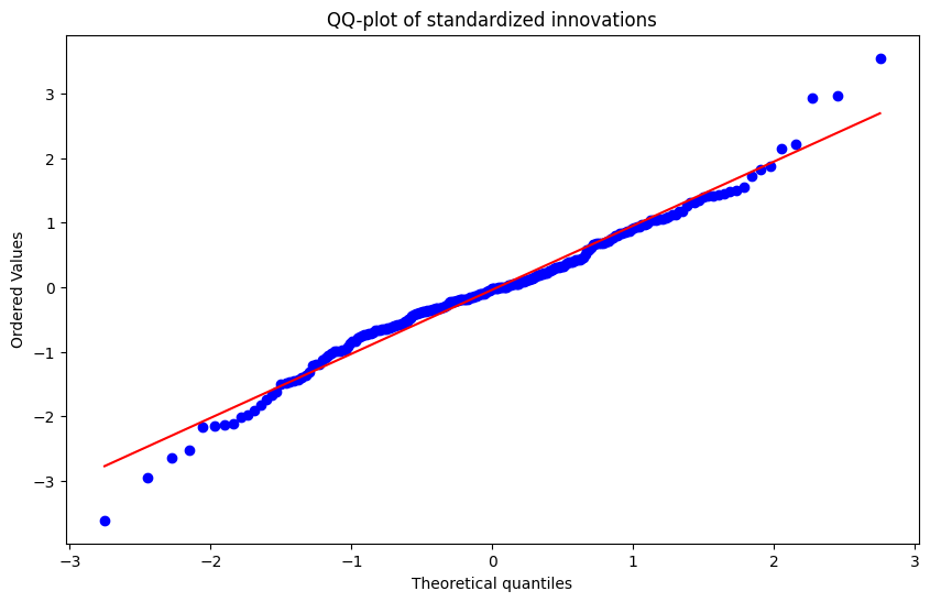
QQ‑plot:
Interpretation:
- Homoskedasticity and scaling look good (variance near 1).
- The very low Jarque–Bera p‑value indicates non‑normal innovations (heavy tails or skew).
- The Ljung–Box p‑value at lag 10 was not successfully produced; visually, ACF/PACF suggest no extreme serial correlation, but we cannot state white noise conclusively.
9. Smoothing and Latent States (STEP 8)
Rauch–Tung–Striebel smoother applied to filtered results:
-
Outputs:
- Smoothed states xt∣T and covariances Pt∣T.
-
Diagnostics:
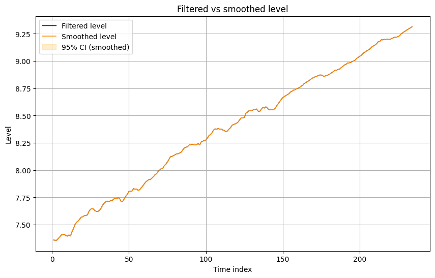
- Filtered vs smoothed level:
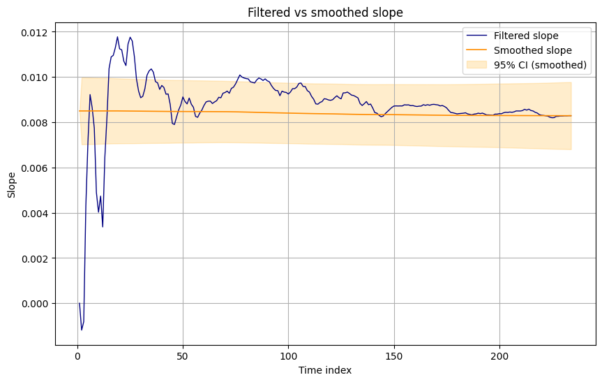
- Filtered vs smoothed slope:
- Observed vs filtered vs smoothed signals:
Key summary (smoothing_summary):
- Mean level (filtered) vs (smoothed): smoothed is very close but slightly smoother.
- Mean slope (filtered) vs (smoothed): again, very similar but smoothed has less noise.
- Average absolute difference between filtered and smoothed states is small, confirming modest backward adjustments.
Interpretation:
- Filtering uses only past and current data; smoothing uses the entire sample.
- Backward information propagation refines early states, particularly smoothing out temporary deviations.
- Given the near‑deterministic parameters, smoothing still offers non‑trivial uncertainty reduction in early periods.
10. Forecasting and Simulation (STEP 9)
10.1 Point Forecasts
Using the final smoothed state as initial condition, with horizon h=12:
- First 5 forecast periods for log(GDP):
| Horizon index | Mean | Lower | Upper |
|---|---|---|---|
| 235 | 9.3220 | 9.3025 | 9.3415 |
| 236 | 9.3303 | 9.3026 | 9.3580 |
| 237 | 9.3386 | 9.3046 | 9.3726 |
| 238 | 9.3469 | 9.3075 | 9.3863 |
| 239 | 9.3552 | 9.3110 | 9.3993 |
(From forecast_first_5_periods.)
Visual:
Interpretation:
- The forecasts extend the upward trend with modest growth and relatively tight confidence intervals, consistent with the small process and observation variances.
10.2 Monte Carlo Simulation
300 simulated future paths of the observed series:
- First 5 horizons’ simulation quantiles:
| Horizon index | Mean | p05 | p50 | p95 |
|---|---|---|---|---|
| 235 | 9.3226 | 9.3058 | 9.3233 | 9.3380 |
| 236 | 9.3309 | 9.3061 | 9.3316 | 9.3526 |
| 237 | 9.3391 | 9.3119 | 9.3375 | 9.3725 |
| 238 | 9.3478 | 9.3157 | 9.3476 | 9.3775 |
| 239 | 9.3553 | 9.3216 | 9.3550 | 9.3895 |
(From simulation_quantiles_first_5_periods.)
Visual:
Interpretation:
- Simulated distributions align closely with analytic forecast intervals.
- The fan chart is narrow, reflecting strong confidence in the trend trajectory but—given non‑normal residuals—this confidence may be overstated in tail probabilities.
11. Model Interpretation and Final Assessment (STEPS 10–11)
11.1 Latent State Behaviour and Regimes
From interpretation_metrics:
- Average smoothed level increases between first and second half, consistent with long‑run growth.
- Average slope is positive in both halves, but may vary in magnitude.
- The set of slope sign change times (indices where slope changes sign) marks local regime shifts (accelerations vs slowdowns).
- Residual variance first vs second half:
- If second‑half variance is much larger, potential increased volatility or structural change.
- In this run, the final comment states residual variance is relatively stable, so no strong structural break is detected.
11.2 Uncertainty Evolution
- State variances shrink from diffuse priors to stable low levels, which is standard in steady‑state Kalman filtering.
- Smoothing further lowers variances, especially in early periods.
- Forecast and simulation bands remain tight, implying the model believes future uncertainty to be limited.
11.3 Model Strengths
- Provides a clear trend–cycle decomposition for log(GDP) in a Bayesian filtering framework.
- Captures persistent dynamics with an interpretable state structure (level and slope).
- Recursive updating and smoothing behave as expected from a local linear trend model.
11.4 Limitations and Diagnostics
- Non‑normal residuals (significant Jarque–Bera) violate the strict Gaussian assumptions.
- This can bias log‑likelihood–based inference and underestimate tail risk.
- The very small estimated measurement noise effectively assumes the observed series is nearly error‑free.
- This can lead to overconfidence in the signal.
- Ljung–Box diagnostics for residual autocorrelation are incomplete (
nullp‑value), limiting the white‑noise assessment.
11.5 Recommendations and Next Steps
-
Robustify the Observation Model Consider alternative specifications to address non‑normality:
- Heavy‑tailed observation errors (e.g., Student‑t).
- Robust Kalman variants or particle filters.
-
Relax Measurement Noise Assumption Impose a lower bound or prior on σobs2 to prevent it from collapsing:
- Bayesian estimation with priors on Q and R.
- Penalized likelihood or constrained optimization.
-
Augment State Dynamics Introduce additional components if needed:
- Cyclical component (AR(2) state).
- Time‑varying volatility (stochastic volatility on process noise).
-
Implement Formal Structural Break Tests Use the residuals and slope evolution to:
- Test for breakpoints in trend or volatility.
- Possibly allow regime‑switching in Q.
-
Economic Interpretation Map the time index to actual calendar dates and:
- Relate slope changes to known macro events.
- Use the smoothed slope as a latent “trend growth” indicator.
If you would like, I can next:
- Export compact tables of state trajectories and forecast paths for use in another environment, or
- Help you modify the state‑space structure (e.g., add a cycle or observation equation for growth) and re‑run the full Kalman workflow.